
Issue # 1 - Why LLM Inference is Different ?
LLM Inference Engineering - The costs, bottlenecks, and physics that make LLM serving a fundamentally different problem.


This is Chapter 1 of an open-source handbook I'm writing on LLM inference at scale (GitHub). If you're building serving infrastructure, this is for you.
Introduction
When I started working on LLM inference, I assumed it would be like regular ML inference - just bigger models. I was wrong ! Everything I knew about ML inference either didn’t apply or actively misled me. The cost structure is different. The bottlenecks are different. The scaling behaviour is different. And the optimisation levers are completely different.
The 100x Problem
Let’s start with the number that should bother you.
Traditional ML inference models like ResNet, BERT, a recommendation model costs roughly $0.001 per request. Latency is 5–20ms. Memory usage is fixed. Batching is trivial. Scaling is linear. It’s a solved problem.
LLM inference costs $0.01–0.10 per request. Latency swings between 100ms and 10 seconds depending on output length. Memory grows during the request. Batching requires a whole new paradigm. Scaling is sub-linear and communication-bound.
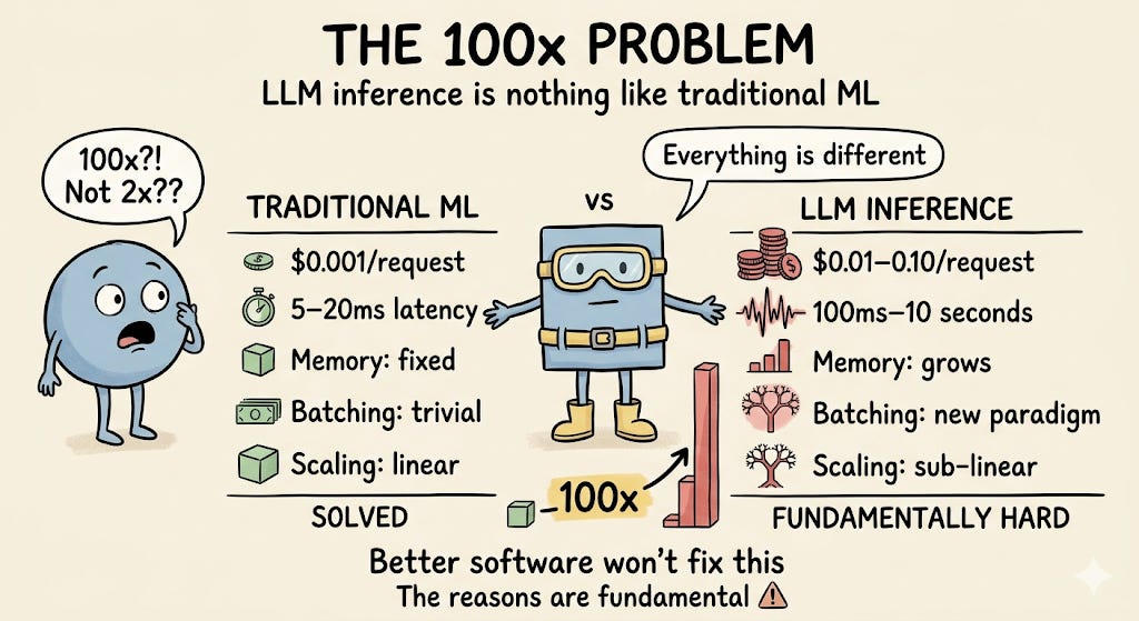
The gap isn’t 2x or 5x. It’s 100x. And the reasons are fundamental — not something better software will fix.
Why LLMs Are Built Differently
The core difference comes down to one word: autoregressive.
Traditional ML inference is a single forward pass. You feed an image into ResNet, data flows through the network once, you get a classification. The time is fixed. The memory is constant. You can batch 100 requests and the cost per request drops.
LLMs work completely differently.
When you ask “What is the capital of France?”, the model doesn’t produce the full answer at once. It generates one token at a time:
“The” → “capital” → “of” → “France” → “is” → “Paris”
Each token is a separate forward pass through the entire model. Token 5 cannot be generated until tokens 1–4 exist. That’s not an engineering limitation to be solved — it’s how autoregressive language models work by design. The probability distribution for each token depends on every token that came before it.
The Weight Reading Problem
Here’s the number that made everything click for me.
Every time the model generates a token, it needs to run a full forward pass. A full forward pass means reading all of the model’s parameters from GPU memory into the compute units. The GPU doesn’t “remember” its weights between operations, every matrix multiply requires loading the weight matrix fresh from memory.
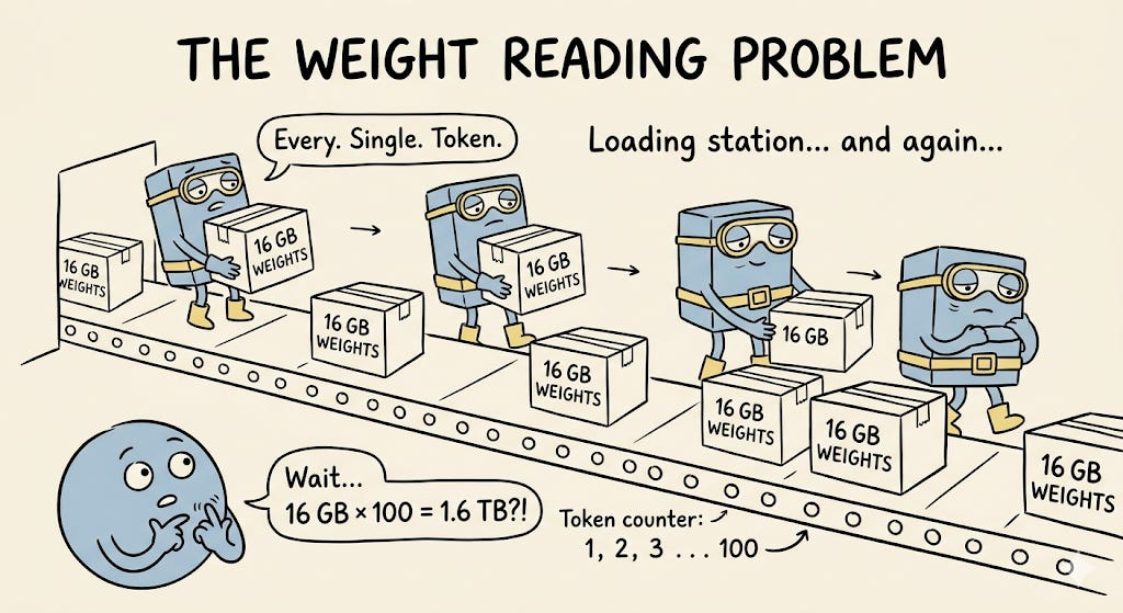
For Llama 3.1 8B generating 100 tokens, that looks like this:
Token 1 → read 16 GB of weights
Token 2 → read 16 GB of weights again
Token 3 → read 16 GB of weights again
… and so on for every token
Total memory reads: 16 GB × 100 = 1.6 TB
And this leads directly to a hard physical ceiling that no software can break.
The Memory Bandwidth Wall
An A100 GPU has 2 TB/s of memory bandwidth. Llama 8B in FP16 weighs 16 GB. So the minimum time to generate one token is:
16 GB ÷ 2 TB/s = 8ms → maximum 125 tokens/second
That’s a hard ceiling. Not a guideline. Not something you can optimise past with clever code.
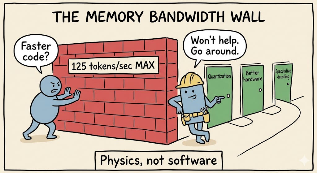
The only ways around this wall are:
Quantization : smaller weights mean fewer bytes to read
Better hardware : more memory bandwidth, not more compute
Speculative decoding : generate multiple tokens per weight read, breaking the sequential bottleneck
Notice what’s not on that list: faster software, smarter scheduling, more efficient attention. Those help with other things, but they don’t move this ceiling.
Two Phases, Two Completely Different Problems
Every LLM request goes through two distinct stages, and they could not be more different.
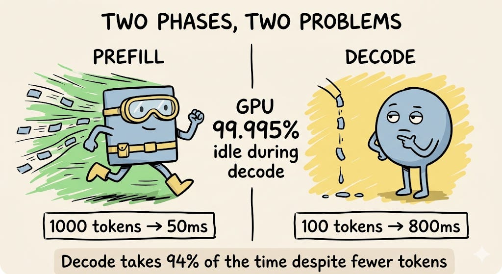
Prefill is when the model processes your entire prompt. All tokens are processed in parallel in a single forward pass. This phase is compute-bound : the GPU is doing massive parallel matrix multiplications and its cores are fully utilised. A 1000-token prompt takes roughly 50ms.
Decode is when the model generates your response, one token at a time. Each token is its own forward pass. This phase is memory-bound : the GPU spends most of its time waiting for data to arrive from memory, not actually computing.
Here’s how idle the GPU actually is during decode:
What the A100 can do: 312 TFLOPS
What it actually does during decode: ~16 GFLOPS
GPU utilisation during decode: 16 ÷ 312,000 ≈ 0.005%
The GPU is 99.995% idle while generating your tokens.
This is why throwing a faster GPU at a decode-bound system barely helps, memory bandwidth scales much slower than raw compute between GPU generations.
Here’s the part that surprises most engineers the first time they see it.
Take a request with a 1000-token prompt generating 100 tokens of output:
Prefill: process 1000 tokens in one pass → ~50ms
Decode: 100 passes × 8ms each → ~800ms
Total: 850ms. Decode is 94% of the time despite processing 10x fewer tokens.
Decode dominates even though it does less work. This single asymmetry drives almost every architectural decision in LLM inference : continuous batching, disaggregated serving, speculative decoding, KV cache management. All of it traces back to this.
Why This Changes How You Think About Optimization
Once you internalize these two constraints, decisions that seemed arbitrary start making sense.
Batching helps decode because processing multiple requests together amortises the weight reads across all of them, increasing arithmetic intensity and moving you toward better GPU utilization.
Quantization helps because INT8 weights are half the size of FP16 weights - fewer bytes to read per token, faster decode.
Speculative decoding is clever because a small draft model proposes multiple tokens, which the large model verifies in parallel - effectively generating multiple tokens per weight read.
Disaggregated serving exists because prefill and decode have completely different hardware profiles. Running them on the same GPU means compromising on both.
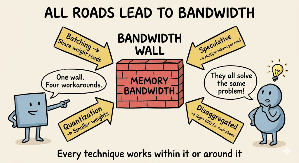
All roads lead back to the same place: memory bandwidth is the wall, and every technique is either working within it or around it.
What’s Next
This was the foundation. Next chapter goes one level deeper.
Module 0.2: Transformer Inference Mechanics — a byte-level walkthrough of how attention actually works during inference, the KV cache math, why grouped query attention exists, and concrete memory access patterns with real numbers.
I’m writing this handbook in public at github.com/harshuljain13/llm-inference-at-scale. If something is wrong, open an issue. If it’s useful, a ⭐ helps others find it.
If a colleague is building LLM serving infrastructure, forward this their way.
 | A guest post by
|